CS 4641 Project
Final Report
Introduction
In today’s world, the average consumer has access to millions of songs at the simple click of a button, a catalog that includes songs that span across eras, artistic expressions, and themes. While this presents music enthusiasts with an exciting opportunity to get more involved with their work, it also presents many challenges when it comes to organizing, classifying, and recommending songs to individuals with varied tastes.
Our team is impressed by the amount of research that has been done in this area, and wants to add to this literature. We have located several similar studies that each test different models, such as Convolutional Neural Networks (CNNs) [1] and Support Vector Machines [2]. We hope to compare and contrast more types of models to create a better genre classification model.
We plan to accomplish this by analyzing a dataset containing 1700 spectrograms derived from songs that are 270-300 seconds in length, and sorted into a hierarchy containing 3 levels of classifications and 16 distinct genres. Due to limitations in the dataset, our research will mainly be limited to English songs.
Problem Definition & Motivation
This project aims to revolutionize music genre classification by leveraging advanced image processing techniques on spectrograms. By translating visual data into numeric representations, we aim to extract crucial features for precise genre classification. Our unique approach includes a comprehensive analysis of various models, such as Convolutional Neural Networks (CNNs) and Support Vector Machines (SVMs), in order to compare and contrast their effectiveness. This classification process is structured to identify if a song belongs to one of nine distinct categories. Through this approach, we seek to not only enhance the accuracy of genre classification, but also to uncover intricate and hidden trends within these categories. This project holds the potential to yield invaluable insights for artists, record labels, and music enthusiasts alike.
Data Collection
Our team utilized the pre-existing dataset consisting of spectrogram images. Our dataset can be found here: https://huggingface.co/datasets/ccmusic-database/music_genre. We refined this dataset with a feature selection algorithm.
The original dataset consists of 1,700 spectrogram images from songs lasting between 270 and 300 seconds. These images, sized at 349x476 pixels, are in JPEG format and represent the spectrograms of music files. Created using Fast Fourier Transform (FFT), these spectrograms map the sound frequencies and intensities over time.
In each spectrogram:
- The X-axis indicates time.
- The Y-axis shows frequency.
- The brightness of each pixel reflects the intensity of sound waves at specific frequencies and times.
Human voices and musical instruments produce unique waveforms. In a spectrogram, these waveforms are decomposed into various frequency sound waves, forming distinct patterns along the Y-axis. The presence and duration of each instrument or voice in the music are captured along the X-axis.
The dataset is categorized into three hierarchical levels:
- First-level classification: Broadly distinguishes between classical and non-classical music.
- Second-level classification: specific genres within the first level, such as classifying a piece as a symphony within the classical genre or as pop within the non-classical genre.
- Third-level classification: Provides finer subcategories such as Teen_pop or pop_vocal_ballads in pop Categories.
First we transformed the image file into gray scale since color does not have any information but intensity does. After that we transformed to Gray scale co-occurance matrix(GLCM)[5] from the image to select contrast, dissimilarity, homogeneity, energy and correlation features.
After some preliminary tests were performed, we found that this set of features was likely not expressive enough to fully encapsulate the properties necessary for comprehensive genre classification. We revisited our data, and decided to implement SciKit-Learn’s Histograms of Oriented Gradients (HoG) as a better feature descriptor. This is a common approach utilized in many image recognition tasks to better compress the feature width while still maintaining the core information about the image. We used 10 orientations, with 10x10 pixels per cell, and 2x2 cells per block to generate the histograms. This resulted in each image being represented by a 1x60720 vector, resulting in an overall compression ratio of 0.3655.
Methods
KMeans (Unsupervised)
On the unsupervised side we used KMeans. Using K-Means helps identify patterns within the dataset, which will help us find similarities and differences across genres. We used this method because it efficiently clusters large datasets, and works with grouping similar spectrograms.
Support Vector Machines (Supervised)
For our Support Vector Machine model, we utilized Scikit-Learn’s C-Support Vector Classification (SVC) which performs better with smaller scaled datasets of around 10,000 entries. Multiclass classification was handled in a one-vs-one schema to best decide on a final category classification. We independently trained two such SVC models to compare the results of the GLCM and HoG features. The hyperparameters of each of these models were optimized using 3-fold cross validation. This was performed using randomized grid search over 50 iterations. Unfortunately, due to limitations with our hardware, we were unable to perform a more comprehensive grid search to better fine tune the parameters.
Random Forests (Supervised)
For our Random Forest model, we utilized Scikit-learn’s Random Forest Classifier. The model was trained on features derived using both GLCM & Correlation and Histogram of Oriented Gradients (HoG) techniques. We split the dataset into 80% for training and 20% for validation. We used RandomizedSearchCV to tune the hyperparameters of our model.
Logistic Regression (Supervised)
For the Logistic Regression model, we utilized Scikit-Learn’s Logistic Regression class to independently train two models, one utilizing the GLCM features and the other the HoG features.
Convolutional Neural Network (Supervised)
One of the supervised learning methods we tried was training a Convolutional Neural Network. We used PyTorch to implement a custom Dataset class for our images to handle the loading and transformation by resizing every image to be 256 x 256 pixels. We then split the data into training (80%) and testing (20%) sets. The architecture itself was quite simple, comprising two convolutional layers, each followed by a max pooling layer. The first layer had 16 filters while the second had 32, and both had a kernel size of 3 and padding of 1. These convolutional layers were followed by two fully connected layers and a dropout layer in order to reduce overfitting. We used Cross-Entropy Loss as our loss function and Stochastic Gradient Descent as our optimization with a learning rate of 0.001, momentum of 0.9, and weight decay of 0.001. We also used Resnet50 as a pre-trained base for our CNN and replaced the last fully connected layer with a dropout layer and a fully connected layer that matched our number of classes.
Results and Discussion
| Model | Feature Set | Precision | Recall | F1-Score |
|---|---|---|---|---|
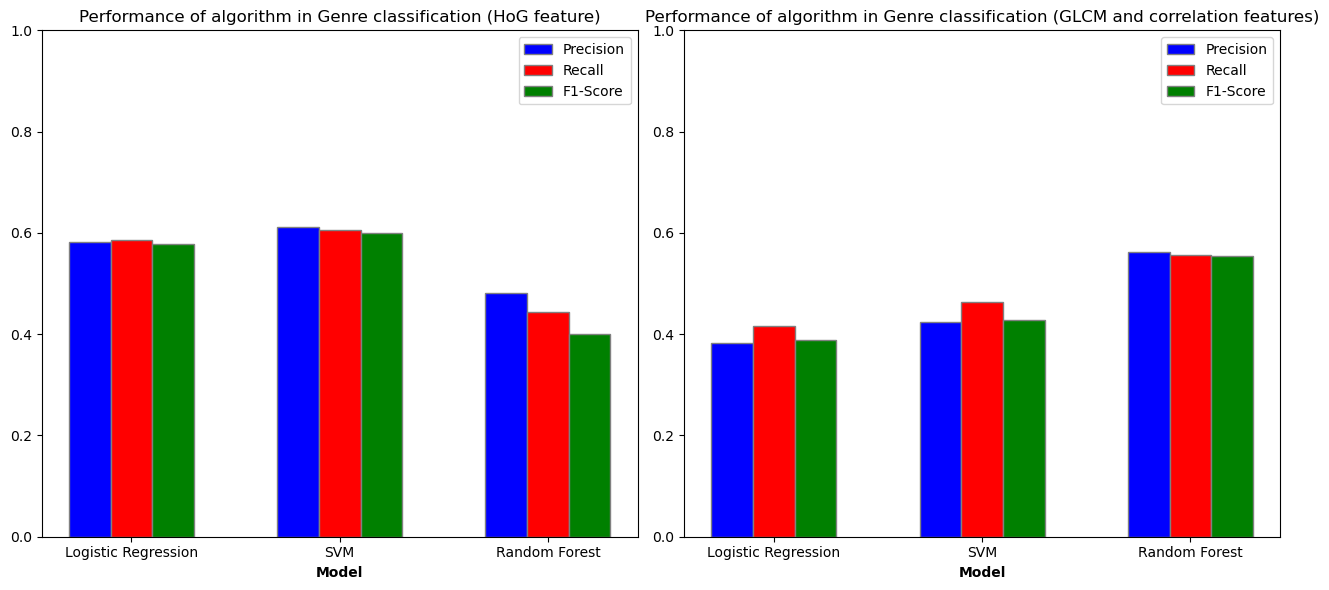
| Logistic Regression | HoG | 0.582380 | 0.586006 | 0.578080 |
| Logistic Regression | GLCM | 0.382263 | 0.416910 | 0.388116 |
| SVM | HoG | 0.611368 | 0.606414 | 0.599056 |
| SVM | GLCM | 0.424060 | 0.463557 | 0.428644 |
| Random Forest | HoG | 0.480725 | 0.443149 | 0.400398 |
| Random Forest | GLCM | 0.561327 | 0.556851 | 0.554355 |
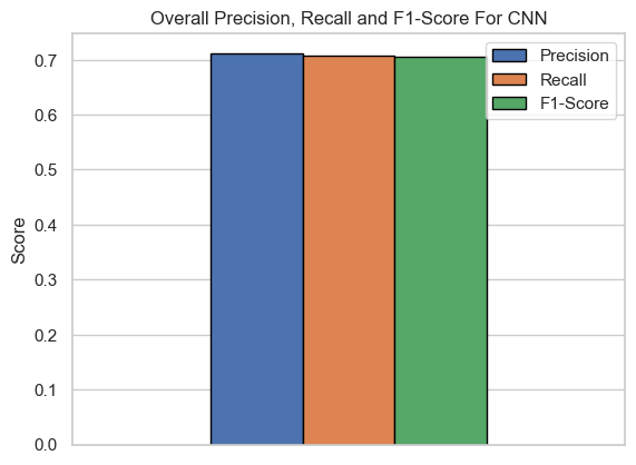
| CNN | Raw Pixels | 0.712410 | 0.710752 | 0.704212 |
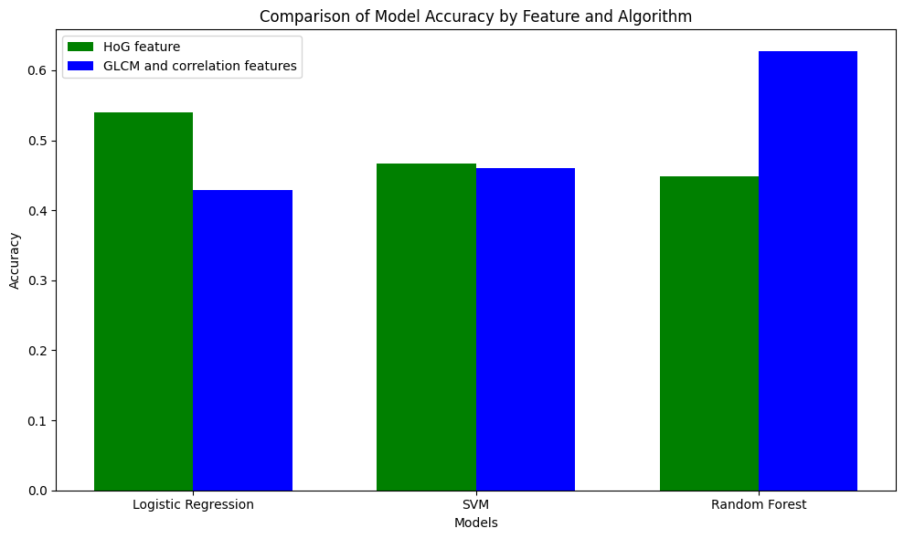
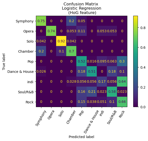
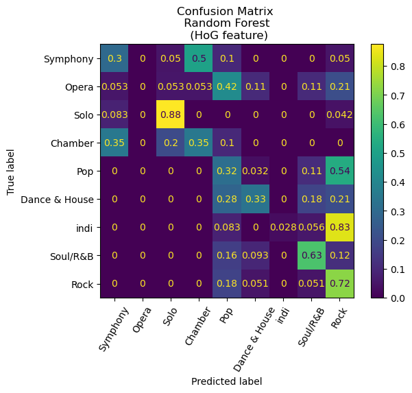
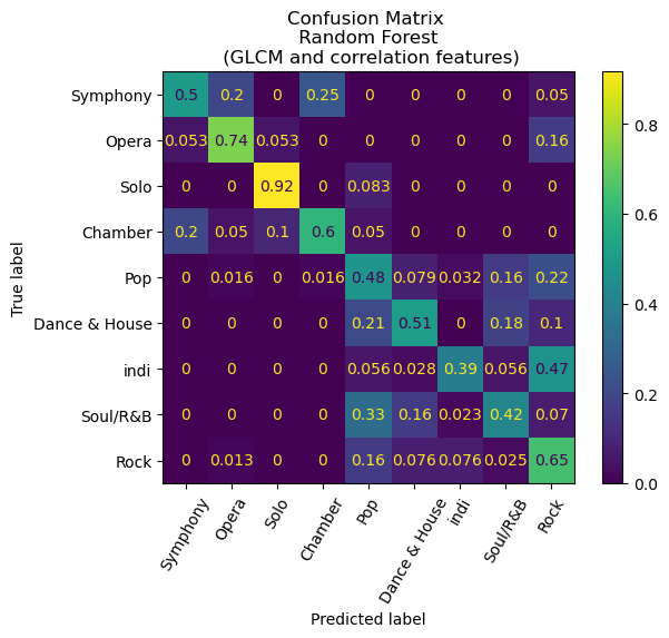
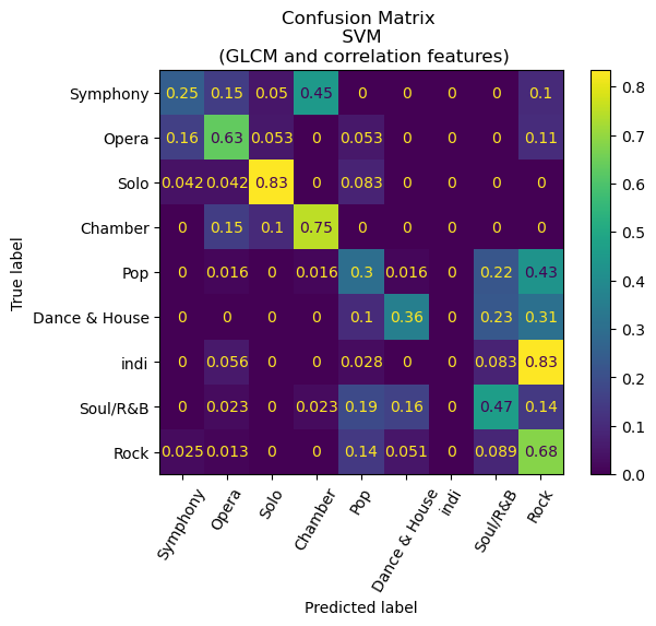
From Table 1, we see that CNN performed the best out of all tested models. Using Resnet50 as a base for our CNN, we were only able to achieve an accuracy of 62.1%, but with our simple convolutional neural network architecture and some hyperparameter tuning, we were able to achieve an accuracy of 71.24%. As we expected, HoG indeed performed as a better feature predictor than GLCM, outperforming in all models (except Random Forest) by an average of 27.4%.
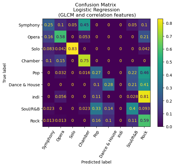
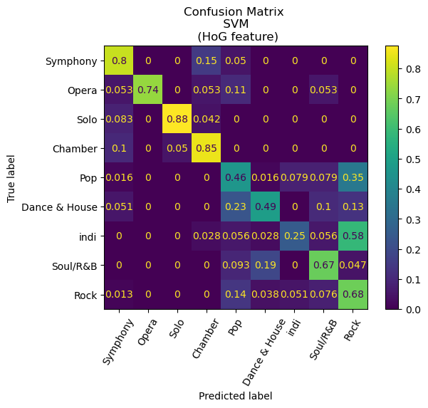
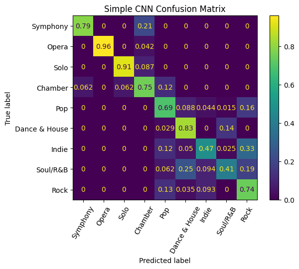
An intriguing finding emerges from the analysis, wherein each of the models exhibits exemplary performance in distinguishing between classical and non-classical songs. The former encompasses genres such as symphony, opera, solo, and chamber, as distinct from pop, dance and house, indie, soul and R&B, and Rock. Remarkably, the confusion matrix for our Convolutional Neural Network (CNN) model manifests a noteworthy outcome, as it demonstrates an absence of misclassifications between classical and non-classical genres.
Additionally, a deeper examination of the confusion matrices reveals a notable pattern among the misclassifications, with a predominant trend of predicting indie songs as rock. Significantly, the CNN model exhibited a misclassification rate of 33% for indie songs, whereas the random forest with Histogram of Oriented Gradients (HoG) model demonstrated a considerably higher misclassification rate of 81%. While there is a certain degree of rationale behind this observation, given the tendency of the indie genre to draw inspiration from rock and other musical forms, a more nuanced exploration is warranted. It is conceivable that the observed misclassification pattern may be influenced by the relatively limited representation of indie songs in our dataset, comprising only 201 entries compared to 401 rock songs. This discrepancy in sample size may result in the model assigning a higher weight to the genre it encounters more frequently, thereby impacting its classification proficiency.
Visualizations of our results can be found below.
Conclusion
In summary, our exploration into genre classification has yielded commendable results. While our findings may not be considered groundbreaking, the notable achievement lies in the high classification accuracy attained by our CNN model. Additionally, our analysis uncovered discernible patterns in music genre classification, shedding light on statistically significant correlations among certain categories and revealing weaker associations in others.
An essential takeaway from this study is the enhanced understanding of the pivotal role of feature engineering. Notably, the integration of Histogram of Oriented Gradients (HoG) led to substantial improvements across the majority of our models. Looking ahead, we envision the potential for more comprehensive insights by revisiting this project with an expanded dataset and increased processing power. The limitations imposed by the relatively modest dataset of around 1700 spectrograms, coupled with the constrained scope of Western music genres, underscore the need for future iterations of this study to encompass a broader musical landscape.
References
- N. M R and S. Mohan B S, “Music Genre Classification using Spectrograms,” 2020 International Conference on Power, Instrumentation, Control and Computing (PICC), Thrissur, India, 2020, pp. 1-5, doi: 10.1109/PICC51425.2020.9362364.
- Costa, Yandre & Soares de Oliveira, Luiz & Koericb, A.L. & Gouyon, Fabien. (2011). Music genre recognition using spectrograms. Intl. Conf. on Systems, Signal and Image Processing. 1 - 4.
- M. Dong, ‘Convolutional Neural Network Achieves Human-level Accuracy in Music Genre Classification’, CoRR, vol. abs/1802.09697, 2018.
- Zhaorui Liu and Zijin Li, “Music Data Sharing Platform for Computational Musicology Research (CCMUSIC DATASET).” Zenodo, Nov. 12, 2021. doi: 10.5281/ZENODO.5676893.
- M. Hall-Beyer, 2007. GLCM Texture: A Tutorial https://prism.ucalgary.ca/handle/1880/51900 DOI:10.11575/PRISM/33280
- V. Bisot, S. Essid and G. Richard, “HOG and subband power distribution image features for acoustic scene classification,” 2015 23rd European Signal Processing Conference (EUSIPCO), Nice, France, 2015, pp. 719-723, doi: 10.1109/EUSIPCO.2015.7362477.
- Y. Panagakis, C. Kotropoulos and G. R. Arce, “Non-Negative Multilinear Principal Component Analysis of Auditory Temporal Modulations for Music Genre Classification,” in IEEE Transactions on Audio, Speech, and Language Processing, vol. 18, no. 3, pp. 576-588, March 2010, doi: 10.1109/TASL.2009.2036813.
Contributions
| Contribution | People Involved |
|---|---|
| Neural Implementation | Siddhant |
| Analysis | Siddhant |
| Visualization, Quantitative Metrics | Soongeol, James |
| Presentation | Joseph |
| Hyperparameter Tuning | James, Anirudh |
| Update Timeline/Contribution Table | Soongeol |
| Tuning Code | Everyone |
| Results | Everyone |