CS 4641 Project
Midterm Report
Introduction
In today’s world, the average consumer has access to millions of songs at the simple click of a button, a catalog that includes songs that span across eras, artistic expressions, and themes. While this presents music enthusiasts with an exciting opportunity to get more involved with their work, it also presents many challenges when it comes to organizing, classifying, and recommending songs to individuals with varied tastes.
Our team is impressed by the amount of research that has been done in this area, and wants to add to this literature. We have located several similar studies that each test different models, such as Convolutional Neural Networks (CNNs) [1] and Support Vector Machines [2]. We hope to compare and contrast more types of models to create a better genre classification model.
We plan to accomplish this by analyzing a dataset containing 1700 spectrograms derived from songs that are 270-300 seconds in length, and sorted into a hierarchy containing 3 levels of classifications and 16 distinct genres. Due to limitations in the dataset, our research will mainly be limited to English songs.
Problem Definition & Motivation
This project aims to classify the genres of songs based on their spectrograms. Using image processing techniques to redefine visual data into numeric data. and extract useful features to classify the music genre. We have three subtasks for classification:
- First-level classification: Broadly distinguishes between classical and non-classical music.
- Second-level classification: specific genres within the first level, such as classifying a piece as a symphony within the classical genre or as pop within the non-classical genre.
- Third-level classification: Provides finer subcategories such as Teen_pop or pop_vocal_ballads in pop Categories.
In developing these classifications, we hope this project can lead into helping to identify trends within genres, which would provide valuable insights for artists, labels, and consumers.
Data Collection
Our team utilized the pre-existing dataset consisting of spectrogram images. Our dataset can be found here: https://huggingface.co/datasets/ccmusic-database/music_genre. We refined this dataset with a feature selection algorithm.
The original dataset consists of 1,700 spectrogram images from songs lasting between 270 and 300 seconds. These images, sized at 349x476 pixels, are in JPEG format and represent the spectrograms of music files. Created using Fast Fourier Transform (FFT), these spectrograms map the sound frequencies and intensities over time.
In each spectrogram:
- The X-axis indicates time.
- The Y-axis shows frequency.
- The brightness of each pixel reflects the intensity of sound waves at specific frequencies and times.
Human voices and musical instruments produce unique waveforms. In a spectrogram, these waveforms are decomposed into various frequency sound waves, forming distinct patterns along the Y-axis. The presence and duration of each instrument or voice in the music are captured along the X-axis.
The dataset is categorized into three hierarchical levels:
- First-level classification: Broadly distinguishes between classical and non-classical music.
- Second-level classification: specific genres within the first level, such as classifying a piece as a symphony within the classical genre or as pop within the non-classical genre.
- Third-level classification: Provides finer subcategories such as Teen_pop or pop_vocal_ballads in pop Categories.
First we transformed the image file into gray scale since color does not have any information but intensity does. After that we transformed to Gray scale co-occurance matrix(GLCM)[5] from the image to select contrast, dissimilarity, homogeneity, energy and correlation features.
Data Preprocessing (Feature Creation & Selection):
Given that we had image data, we needed to convert it into a format that works with traditional Machine Learning algorithms like K-Means. In order to do this, we used PIL and Numpy to convert the image into an array of floats. We then extracted several features from this array of floats, including the mean value, contrast, dissimilarity, homogenity, energy, correlation.
Methods
The methods used are Principal Component Analysis (PCA), and the unsupervised learning model we used was K-Means clustering. Using K-Means helps identify patterns within the dataset, which will help us find similarities and differences across genres. We used this method because it efficiently clusters large datasets, and works with grouping similar spectrograms. In this project we used PCA for visualization purposes, rather than feature selection. By reducing the high dimensional spectrogram data to three dimensions. PCA enables the effective visual representation of the data. This helps in our understanding of the underlying structures and relationships. PCA works by transforming the data into a smaller number of uncorrelated variables or principal components. The combination of PCA and K-Means helps us uncover patterns within the music genres, which can be used in the future for adding music recommendation systems, trend analysis, etc.
Quantitative Metrics
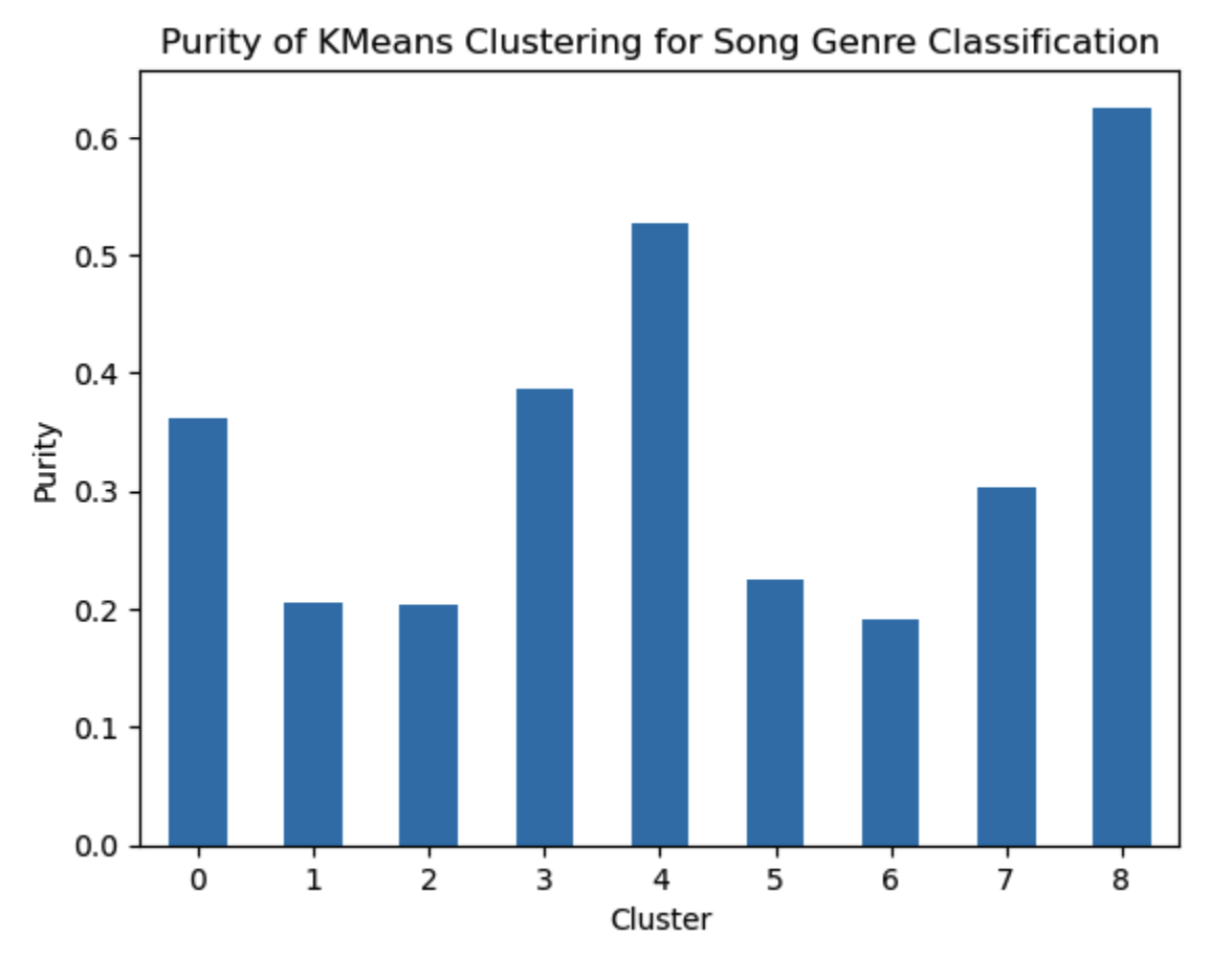
As can be seen in Figure 1 below, the purity scores for the eight clusters were lackluster, with four of the clusters having scores near 0.2 and all overall average purity of just above 0.25. We can note silhouette scores for varying number of clusters: 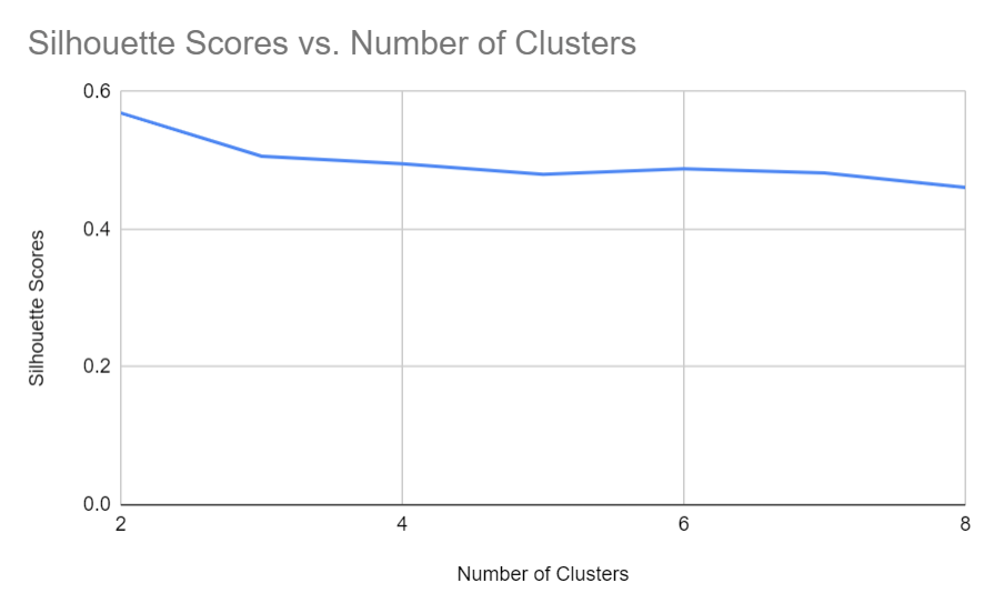
We see the best clustering performance when dividing into two clusters (ideally classical and non-classical), but even with eight clusters there is still a relatively poor performance.
Analysis
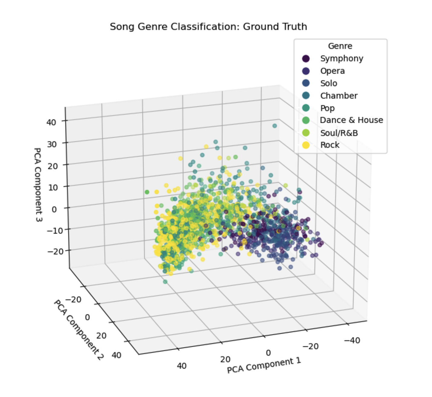
As can be seen in Figure 2 down below (ground truth), we see some distinctions between the classical genres (symphony, opera, solo, and chamber) and the non-classical (pop, dance & house, soul/R&B, and rock), with the former occupying mostly the closer bottom-right octant of the graph in the displayed orientation. The latter genres seem to have a much larger spread, which is not surprising given the larger range in musical techniques and styles among these genres when compared to classical music. This visualization was generated using PCA which reduced the total number of features down to three from over 700.
As discussed above in the quantitative metrics section, we saw that the clustering generally performed pretty poorly, with low purity scores and a low silhouette score even for just two clusters. Unsurprisingly, we do not see any trends within the clusters as in Figure 3 there is no semblance of grouping of the clusters that reflects the distinctions we noted above. As we will discuss in the next section, there is significant room for growth in our feature selection, which will hopefully help with both the supervised learning methods and also improving our clustering.
Visualizations

Future Work
There is still significant room for improvement to make this project a viable genre classifier. Going forward, we plan to focus our work in two main areas: improving our feature selection process and improving our models.
Right now, our feature selection is quite limited, and does not do a great job of separating the data into distinct genre classification. Based on our current research, we have decided to experiment with using histograms of oriented gradients (HoG)[6] for our classification. This is a common feature reduction process used in image recognition, which we hope will translate well to the spectrogram images included in the dataset. However, this will also greatly increase complexity compared to our current features, so we may need to use PCA[7] to reduce the dimensions of the HoG features further.
Furthermore, we are going to branch into using supervised learning techniques for the second half of this project. These techniques will take advantage of the fact that our data is already labeled, and use these labels to better learn how to classify the songs. So far, we have identified five different models we would like to experiment with: logistic regression, support vector machines (SVMs), random forests, gradient boosting, and convolutional neural networks (CNNs). Each of these should give dramatically better results than our current clustering techniques.
References
- N. M R and S. Mohan B S, “Music Genre Classification using Spectrograms,” 2020 International Conference on Power, Instrumentation, Control and Computing (PICC), Thrissur, India, 2020, pp. 1-5, doi: 10.1109/PICC51425.2020.9362364.
- Costa, Yandre & Soares de Oliveira, Luiz & Koericb, A.L. & Gouyon, Fabien. (2011). Music genre recognition using spectrograms. Intl. Conf. on Systems, Signal and Image Processing. 1 - 4.
- M. Dong, ‘Convolutional Neural Network Achieves Human-level Accuracy in Music Genre Classification’, CoRR, vol. abs/1802.09697, 2018.
- Zhaorui Liu and Zijin Li, “Music Data Sharing Platform for Computational Musicology Research (CCMUSIC DATASET).” Zenodo, Nov. 12, 2021. doi: 10.5281/ZENODO.5676893.
- M. Hall-Beyer, 2007. GLCM Texture: A Tutorial https://prism.ucalgary.ca/handle/1880/51900 DOI:10.11575/PRISM/33280
- V. Bisot, S. Essid and G. Richard, “HOG and subband power distribution image features for acoustic scene classification,” 2015 23rd European Signal Processing Conference (EUSIPCO), Nice, France, 2015, pp. 719-723, doi: 10.1109/EUSIPCO.2015.7362477.
- Y. Panagakis, C. Kotropoulos and G. R. Arce, “Non-Negative Multilinear Principal Component Analysis of Auditory Temporal Modulations for Music Genre Classification,” in IEEE Transactions on Audio, Speech, and Language Processing, vol. 18, no. 3, pp. 576-588, March 2010, doi: 10.1109/TASL.2009.2036813.
Proposed Timeline
This timeline is subject to change. A more detailed version can be found here.
| TASK TITLE | TASK OWNER | START DATE | DUE DATE |
|---|---|---|---|
| Project Proposal | |||
| Introduction & Background | James DiPrimo | 9/27/2023 | 10/6/2023 |
| Problem Definition | Anirudh Ramesh | 9/27/2023 | 10/6/2023 |
| Methods | Siddhant Dubey | 9/27/2023 | 10/6/2023 |
| Timeline | Soongeol Kang | 9/27/2023 | 10/6/2023 |
| Potential Results & Discussion | Joseph Campbell | 9/27/2023 | 10/6/2023 |
| Video Recording | Siddhant Dubey | 9/27/2023 | 10/6/2023 |
| GitHub Page | Siddhant Dubey | 9/27/2023 | 10/6/2023 |
| Model 1 (GMM or K-means) | |||
| Data Sourcing and Cleaning | Siddhant Dubey and Anirudh Ramesh | 10/7/2023 | 10/13/2023 |
| Model Selection | Everyone | 10/13/2023 | 10/16/2023 |
| Data Pre-Processing | Siddhant Dubey and Anirudh Ramesh | 10/16/2023 | 10/23/2023 |
| Model Coding | Siddhant Dubey and Anirudh Ramesh | 10/23/2023 | 10/30/2023 |
| Visualizations | James | 10/30/2023 | 11/2/2023 |
| Quantitative Matrics, Analysis (Results Evaluation) | Joseph | 10/30/2023 | 11/2/2023 |
| Describe data set, revise, update timeline/contribution table (Mid report) | Kang | 10/31/2023 | 11/3/2023 |
| Midterm Report | Everyone | 10/31/2023 | 11/3/2023 |
| Model 2 (CNN) | |||
| Model Coding | Siddhant Dubey and Anirudh Ramesh | 10/28/2023 | 11/4/2023 |
| Results Evaluation | Everyone | 11/5/2023 | 11/8/2023 |
| Visualizations | James | 11/5/2023 | 11/8/2023 |
| Quantitative Matrics, Analysis (Results Evaluation) | Joseph | 11/5/2023 | 11/8/2023 |
| Describe data set, revise, update timeline/contribution table (Mid report) | Kang | 11/6/2023 | 11/9/2023 |
| Analysis | Joseph | 11/6/2023 | 11/9/2023 |
| Model 3 (SVMs) | |||
| Midterm Report | Everyone | 11/3/2023 | 11/11/2023 |
| Model Coding | Soongeol Kang, James DiPrimo | 11/11/2023 | 11/18/2023 |
| Results Evaluation | Anirudh Ramesh | 11/18/2023 | 11/21/2023 |
| Analysis | Joseph Campbell | 11/19/2023 | 11/22/2023 |
| Model 4 (Random Forests) | |||
| Model Coding | James DiPrimo, Anirudh Ramesh | 11/15/2023 | 11/22/2023 |
| Results Evaluation | Siddhant Dubey | 11/20/2023 | 11/23/2023 |
| Analysis | Soongeol Kang | 11/21/2023 | 11/24/2023 |
| Evaluation | |||
| Model Comparison | Everyone | 11/29/2021 | 12/4/2021 |
| Presentation | Everyone | 12/1/2023 | 12/6/2023 |
| Recording | Everyone | 12/6/2021 | 12/7/2021 |
| Final Report | Everyone | 12/2/2021 | 12/8/2021 |
Contribution Table
| Contribution | Person |
|---|---|
| Introduction | James |
| Problem Statement | Anirudh |
| Methods | Siddhant |
| Potential Results | Joseph |
| Proposed Timeline | Soongeol |
| Finding Datasets | Everyone |
| Finding Papers | Everyone |
| Contribution 2 | Person |
|---|---|
| pick data pre processing method | Anirudh, Siddhant |
| implement algorithm | Anirudh, Siddhant |
| quantitative metrics | Joseph |
| analysis of algorithm | Joseph |
| visualizations | James |
| Next steps | James |
| describe data set | Soongeol |
| revise references, problem motivation and identification | Soongeol |
| update timeline/contribution table | Soongeol |
| results | Everyone |